02 / Mechanism

How the metasurface functions as a reservoir

The device is easiest to understand as a physical reservoir rather than as a conventional trainable optical neural network. The substrate supplies a shared communication fabric, a nonlinear threshold response, and a finite memory of the previous pulse. Once those three conditions coexist, a simple downstream readout can exploit the resulting state space.^{[1] [4]}

Model Evidence

quasi-BIC

shared high-Q mode enabling long-range collective coupling

Pth

near-threshold operation creates the useful nonlinear regime

Interpretation

Why this is more than a linear optical filter

The output depends on spatial pump pattern, delay history, and operating point in a way that expands the input into a richer physical state. That is the operational reason the reservoir framing is appropriate here.^{[5] [6]}

Backbone

Collective optical mode across the lattice.

Threshold

Gain saturation and lasing onset.

Memory

Finite state retained between pulses.

02 / Components

Mechanism components

The mechanism can be read as four linked components: collective backbone, pump-defined nodes, thresholded response, and finite temporal memory.

Ideal BIC

Mode in the radiation continuum with vanishing leakage due to symmetry or interference.

Quasi-BIC

Slightly leaky version that preserves high Q while remaining experimentally addressable.

Role here

Creates the shared optical backbone that allows distant pumped spots to interact through the same metasurface.^{[2] [3]}

Quasi-BIC physics provides the communication fabric

The quasi-BIC mode stores light unusually well while staying weakly accessible. In this context that matters because it lets the chip support collective states spanning separated pumped regions rather than only local nearest-neighbor behavior.^{[2] [3]}

Field confinement strengthens threshold behavior.
Long-range coupling allows pump-defined nodes to interact through the same lattice.
Weak leakage keeps the mode usable in experiment.

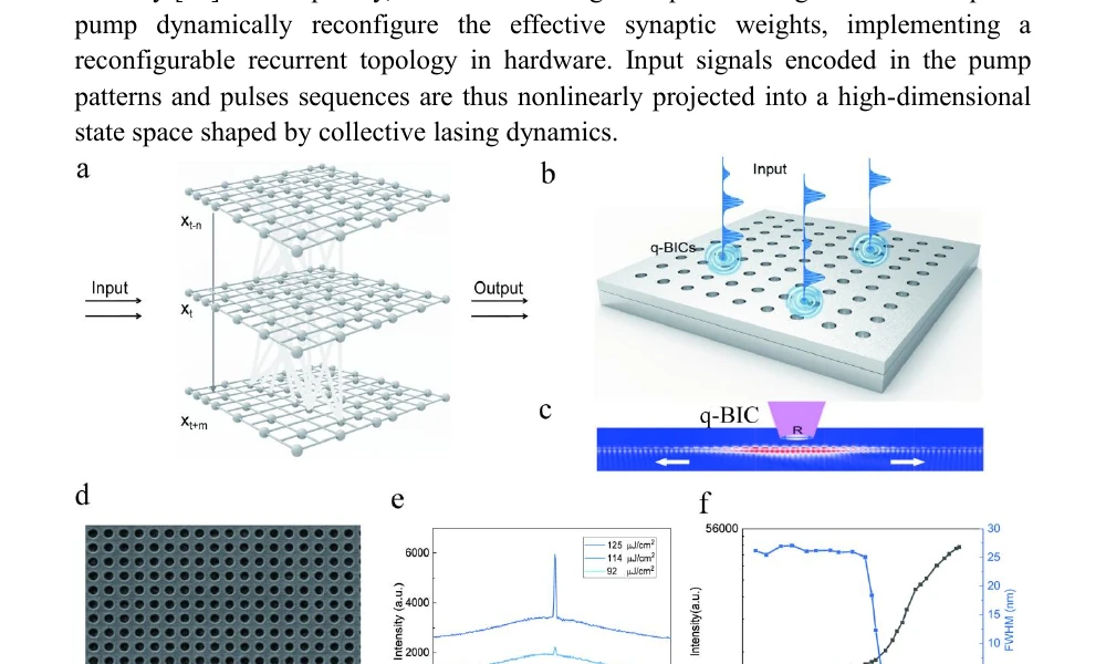
Figure 1 from the paper showing operating principle, device, and threshold behavior

Pump geometry defines virtual nodes

The network is not fabricated as permanent islands. The pump pattern selects which regions are above threshold, which links are emphasized, and which collective supermodes dominate, so the effective topology is reconfigured at the pump plane rather than by storing weights on-chip.^[1]

Node count and spacing are operating-condition choices.
Anisotropy means equal total power does not imply equal internal state.
The metasurface remains the shared computational medium.

Figure 1 threshold region for the active quasi-BIC microlasers

Lasing threshold provides the nonlinear regime

Below threshold, responses are weak and broad. Near threshold, the device moves into a sharply different regime. That regime change supplies the activation-like nonlinearity a useful reservoir needs.^[1]

Threshold crossing is the critical nonlinear event.
Gain saturation prevents the device from behaving like a simple linear filter.
The most useful operating region sits near, but not too far above, threshold.

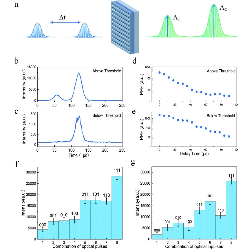
Figure 3 from the paper showing temporal response and paired-pulse facilitation

Residual carriers create short-lived analog memory

The second pulse depends on the first because the gain medium has not fully relaxed. In the paper, paired-pulse facilitation remains visibly significant out to roughly 80 ps in the above-threshold case, which is why the system can process sequences rather than only static patterns.^[1]

Memory is local to the gain medium but visible at the system level.
Delay changes the trajectory, not only the total energy.
This is the ingredient that makes the device recurrent rather than merely static.

Summary

The substrate becomes computational when the three ingredients overlap

The important point is not any single ingredient in isolation. The device becomes interesting when the quasi-BIC backbone, thresholded lasing response, and residual-state memory all coexist under the same pump-defined operating point.

Without the backbone, the nodes are mostly isolated emitters.
Without thresholding, the system remains close to a linear filter.
Without memory, the device is a static nonlinear mapper rather than a recurrent substrate.

Important distinction

The chip is fixed, but the computation is reconfigurable because the pump determines which parts of the chip participate and how the shared modes are excited.

03 / Device

Device details and reservoir abstraction

The device stack matters because it explains both the reconfigurability and the present integration limits. The reservoir abstraction matters because it is the least misleading description of the computation.

Device stack

Etch-free active metasurface

150 nm ZEP520A patterned polymer on an intact 80 nm quasi-2D perovskite film on thin ITO-coated glass.^[1]

Footprint

About 100 x 100 um^2

Compact enough to demonstrate the mechanism clearly, still far from a systems-ready architecture.

Pump

400 nm femtosecond excitation

The paper uses a 100 fs Ti:Sapphire-derived pump at 1 kHz. That is suitable for proof-of-principle work, not yet a deployment model.^[1]

Anisotropy

Unequal axes create directed behavior

Coupling along Gamma-X is stronger than along Gamma-M, so equal total power can still create different internal states.

Encode

Translate bits, image slices, or delayed pulses into a spatial and temporal pump pattern.

Mix

Let quasi-BIC supermodes, gain competition, and recovery dynamics reshape the state.

Read out

Measure integrated intensity or the richer spectral signature of the resulting transient.

Train lightly

Keep the substrate fixed and train only the downstream readout, which is the standard reservoir-computing move.^{[4] [5]}

Paper language

Relative timing and spatial arrangement dynamically reconfigure effective synaptic weights.^[1]

Technical translation

The effective weights are emergent and operating-condition dependent. They are not stored parameters in the way a digital model stores weights.

04 / Model

Operating-point model

This is a qualitative reservoir model, not a microscopic fit to the device. Its job is narrower: show how coupling, pulse spacing, pump level, and spatial pattern move the substrate between weak, useful, and overdriven regimes.

What to do with this panel

1. Choose a pump pattern

Pick which of the three virtual nodes are driven so you can compare distributed excitation against localized excitation.

2. Sweep delay and pump

Shorter delay preserves more residual state; pump near threshold creates the most informative nonlinear region.

3. Read the outputs

Use the chart, PPF proxy, and mode mixture together. The point is to identify regime changes, not to predict benchmark accuracy.

Coupling 0.62

Higher coupling increases shared-state mixing and reduces node independence.

Pulse delay dt 52 ps

Shorter delays leave more residual carrier population from pulse 1.

Pump intensity 1.18 x Pth

Near threshold is the productive operating region. Too far above it becomes harder to control.

Spatial pump pattern

These three-bit motifs stand in for the pump patterns discussed in the paper.

PPF proxy1.00x

Peak total output0.00

Dominant supermodemu1

State-space richnessmedium

Preset operating points

Adjust coupling, delay, and pump to move between weak mixing, productive recurrence, and overdriven behavior.

Under the hood, the model tracks a carrier-like state and an intensity-like output at each node with delayed coupling between nodes. It is deliberately coarse so the operating logic is visible.

Current reading

Operating regime Reservoir window

Pump and coupling are in a useful middle region.

Memory behavior Usable carry-over

Pulse 2 is still affected by pulse 1.

Coupling character Mixed collective

Nodes interact without fully locking together.

Pattern interpretation Three driven nodes

Distributed pumping lets you compare collective and localized modes.

How to read the plot

The orange trace is total output. The colored traces are node-level outputs. Productive settings show a clear second-pulse dependence without collapsing into one dominant locked response.

Next adjustment

Start from the reservoir window preset, then shorten delay to strengthen memory and lower coupling to test how much collective behavior you really need.

Transient output

Node A Node B Node C Total

Proxy supermode mixture

mu1 / collective

mu2 / antisymmetric

mu3 / localized

The state is projected onto three simple basis modes so you can see whether the response is dominated by a shared collective mode, an antisymmetric split, or a more localized pattern. The diagnostic value is comparative, not absolute.